Video 1: For those of you who don't have the time or patience to read through my last two blog entries, this video will serve as a short (10 minute) summmary of the content that follows in the blog.
Introduction
Howdy Again All,
So in my last blog, I discussed the process of modeling and analyzing the attitude dynamics of a rigid, orbital spacecraft via a linearized approximation model. At the end of that blog I remarked on the necessity of modeling the entire spacecraft properly, in a nonlinear fashion. Well, that modeling and analysis is what I hope to discuss in this blog. Essentially, I will be modeling the same spacecraft, with the same moment input at approximately 15 seconds in time while utilizing the three nonlinear equations of motion of our spacecraft. If this sounds interesting to you, or if you just want to numb your brain with some abstract mathematical goodness, feel free to read on.
So in my last blog, I discussed the process of modeling and analyzing the attitude dynamics of a rigid, orbital spacecraft via a linearized approximation model. At the end of that blog I remarked on the necessity of modeling the entire spacecraft properly, in a nonlinear fashion. Well, that modeling and analysis is what I hope to discuss in this blog. Essentially, I will be modeling the same spacecraft, with the same moment input at approximately 15 seconds in time while utilizing the three nonlinear equations of motion of our spacecraft. If this sounds interesting to you, or if you just want to numb your brain with some abstract mathematical goodness, feel free to read on.
Building the Nonlinear Models
So we should address first things first. If you recall from my previous blog, the attitude dynamics and kinematics of an orbital spacecraft can be modeled with three equations of motion. These are reproduced in equations 1 through 3 for reference.
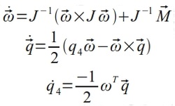
Equations 1 - 3: This set of equations model the changes in angular velocity (w_dot), the quaternion vector (q_dot), and the quaternion scalar (q4_dot) respectively.
If these equations look foreign to you, or you are unfamiliar with the nomenclature being used, I ask you to refer to my previous blog entry, and the nomenclature section therein for reference. I have already described the variables being employed and would rather not reproduce that content for this blog. It is going to be long enough as it is.
Since we know the equations of motion for our particular spacecraft, as well as the mass properties matrix, and the initial state (initial spin conditions), we can actually model these equations directly in Simulink via a series of integration models. For our nonlinear spacecraft model, we do not need to construct a state-space model of the A, B, C, and D matrix form since we are not modeling a linear system. Rather, we will be constructing our own nonlinear plant via a user-defined subsystem block in Simulink. This subsystem block will take a single 7 x 1 input vector (x_dot vector) and output our state variables as three separate vectors (w, q, and q4) after a series of integration loops. As such, our subsystem will utilize three base models, all encapsulated in the same plant. There will be one model for equation of motion. So let's first study the w_dot equation of motion in figure 1.
Since we know the equations of motion for our particular spacecraft, as well as the mass properties matrix, and the initial state (initial spin conditions), we can actually model these equations directly in Simulink via a series of integration models. For our nonlinear spacecraft model, we do not need to construct a state-space model of the A, B, C, and D matrix form since we are not modeling a linear system. Rather, we will be constructing our own nonlinear plant via a user-defined subsystem block in Simulink. This subsystem block will take a single 7 x 1 input vector (x_dot vector) and output our state variables as three separate vectors (w, q, and q4) after a series of integration loops. As such, our subsystem will utilize three base models, all encapsulated in the same plant. There will be one model for equation of motion. So let's first study the w_dot equation of motion in figure 1.
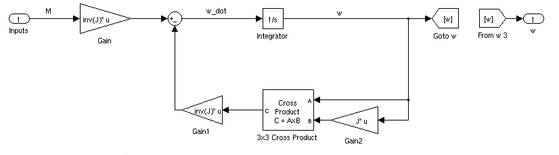
Figure 1: Simulink model of w_dot spacecraft equation of motion, used in nonlinear spacecraft plant in final simulation model.
Observance of figure 1 shows that the angular velocity vector, denoted by the path labeled w, is calculated via the summation of the input moments and the previous w vector crossed with itself. In other words, the angular velocities are reliant upon the spacecraft state at the previous time step as well as whatever moment is currently being input to the system. Already we see a mathematical difference between this model and the linearized model utilized in my previous blog. That model calculated w solely from the input moment scaled by the inertial matrix. This model, however, takes into account the previous behavior of the system thus providing a more robust model.
This complexity is upheld in the calculation of the quaternion vector, depicted in figure 2.
This complexity is upheld in the calculation of the quaternion vector, depicted in figure 2.
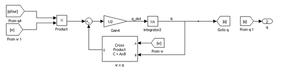
Figure 2: Simulink model of q_dot spacecraft equation of motion, used in nonlinear spacecraft plant in final simulation model.
The nonlinear quaternion vector model sums the product of the angular velocity and q4 with the previous quaternion vector state crossed with omega. Thus, our nonlinear model calculates the quaternion vector, or attitude of the spacecraft, based on the quaternion scalar, the angular velocities (w), as well as the previous quaternion vector state from the prior time step. We see, therefore, that the attitude of the spacecraft is reliant upon the entire state vector, w, q, and q4, rather than simply w as it was in the linear model. So, once again, we have a more comprehensive model of the spacecraft behavior than we did with the linearized system.
Let's take a peak at the quaternion scalar (q4) depicted in figure 3.
Let's take a peak at the quaternion scalar (q4) depicted in figure 3.
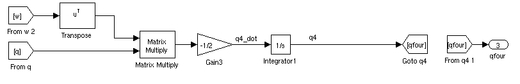
Figure 3: Simulink model of q4_dot spacecraft equation of motion, used in nonlinear spacecraft plant in final simulation model.
The quaternion scalar, oddly enough, does not require a feedback loop as the previous two equations of motion did. In other words, the quaternion scalar is independent of the value of the quaternion scalar from the previous time step, sort of. The quaternion scalar does get utilized to calculate the quaternion vector, which is then utilized to calculate the next quaternion scalar as depicted via the matrix multiplication on the left hand side of the model. So, while the quaternion scalar is not directly dependent upon itself, we do see that it is coupled to the other state variables that are dependent upon it. And, hence we see the cross-linked, nonlinear nature of our system that we discussed in the previous blog.
This shows that the full model of the spacecraft motion is much more comprehensive than the linear approximation. Perturbations to the system are fed into the model via omega (w), but the resulting reaction has a ripple effect throughout the model where each change to a state variable causes further changes to the other state variables. Roughly speaking, this is what is known as a positive feedback loop (though not exactly) due to the self-propagating sensitivity of the state variables.
When we combine all three equations of motion into one plant, we can implement that plant into an overall simulation similar to that utilized to analyze our linear system as depicted in figure 4.
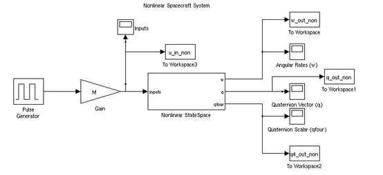
Figure 4: Final nonlinear spacecraft simulation model. Note that the three equation of motion submodels depicted in figures 1 through 3 are encapsulated in the Nonlinear State Space subsystem block in the center of the model. Each equation of motion outputs to its own port from the state space block.
So now that we have a comprehensive, nonlinear model of our spacecraft behavior, we can compare the response of the system to the same impact moment that was enacted upon the linearized spacecraft in my first blog. Theoretically, we should see a much more complicated sensitivity in the system, since the state variables of the system are so reliant upon one another.
Analysis of Results
To reiterate, I ran the same input model for the nonlinear system as I did for the linear system in the last blog. This involved using a pulse generator to enact a 1 second moment impulse on the spacecraft at 15 seconds. The moment induced on the spacecraft was described by the vector M = [5; 1.7; 2.2] Nm, and it is depicted graphically in figure 5.
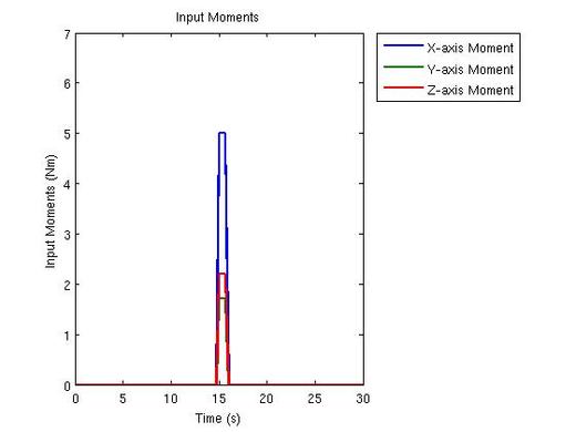
Figure 5: Three input moments were fed into both our linear and nonlinear systems. This is reflected in the M gain block imposed on the pulse generator in each Simulink model.
Based on the models depicted in the previous section, we would expect this moment to affect, primarily, the spin rates of the spacecraft. In figure 6, I plotted up the linear response to this input moment as well as the nonlinear response.
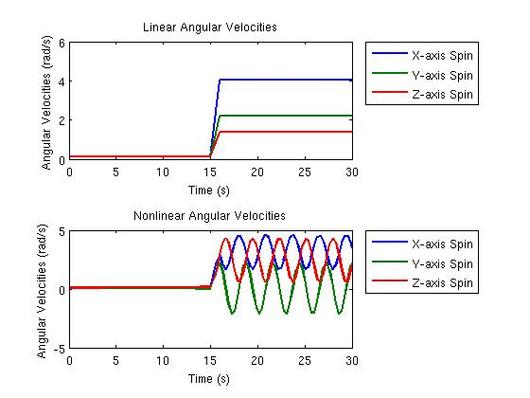
Figure 6: The linear and nonlinear responses of the angular velocities to the moments enacted upon the idealized rigid spacecraft model.
Those plots reveal the underlying complexities of the nonlinear model. In the linear system, we see the typical increase in the angular velocity that is proportional to the input moments. But if we look at the nonlinear system we actually see an oscillating response to the input moment. This occurs, in part, due to the feedbak loop in the angular velocity equation of motion. Since the rate of change of angular velocities relies on the negative addition of the cross product of the previous angular velocity, we end up with a reduction in the next angular velocity . This trend occurs for a spell, until a certain threshold is crossed and the cross product component induces a positive feedback. In other words, the negative cross product component forces the system to oscillate about a particular value.
These are the inertial effects of the body acting on the system. Since we have moments of inertia about each body axis, the mass of the body itself resists the change in direction and magnitude of the angular velocity. This is Newton's first law applied. The inertial properties of the spacecraft are helping to damp the change in angular velocities, thus preventing them from growing uncontrollably. This results in an oscillating system in which the angular velocities wobble about specific values.
This behavior is also reflected in the quaternion vector response depicted in figure 7.
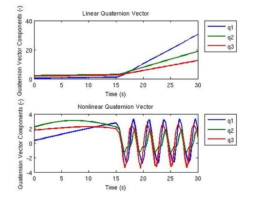
Figure 7: The linear and nonlinear responses of the quaternion vector to the moments enacted upon the idealized rigid spacecraft model.
The quaternion vector response in the nonlinear system varies significantly from the linear response. If you recall, the linear quaternion vector response relied almost entirely upon the scaled angular velocities. Studying the nonlinear quaternion vector model reveals that the quaternion response is now reliant upon both the angular velocity response as well as previous attitude (quaternion vector) and quaternion scalar. The angular velocity, as we discussed, wobbles about some steady values due to the negative cross product component of equation of motion. This effect, combined with the negative cross product between the previous angular velocities and quaternion vector components, results in an oscillating attitude. Essentially, since the spacecraft is tumbling around all three body axes, the attitude is fluctuating between a positive orientation and a negative orientation with respect to the inertial frame.
In the attached video, I discuss how this oscillation in the attitude results in the fluctuations in the angular rates. This is actually backwards and I need to clarify that misinformation now. In fact, the spacecraft is spinning due to the induced moments. However, the off-axis moments of inertia oppose this change in velocity thus resulting in spin rates about each axis that fluctuate between positive and negative. These spin rates cause the attitude of the spacecraft to change in such a manner that it is sometimes pointed in a "positive direction" and sometimes pointed in a "negative direction." So the state variable coupling still exists, the relationship is just reversed from the way it was described orally in the video.
Either way, this response illustrates just how nuanced the nonlinear system is. The physical properties of the spacecraft, the mass properties, actually affect the attitude and spin response of the spacecraft. These effects are reflected via the nonlinear plots, whereas they are mostly lost (serving only to act as a rate multiplier) in the linear model.
Finally, the effects of the oscillating quaternion and angular velocities create a similarly complex response in the quaternion scalar depicted in figure 8.
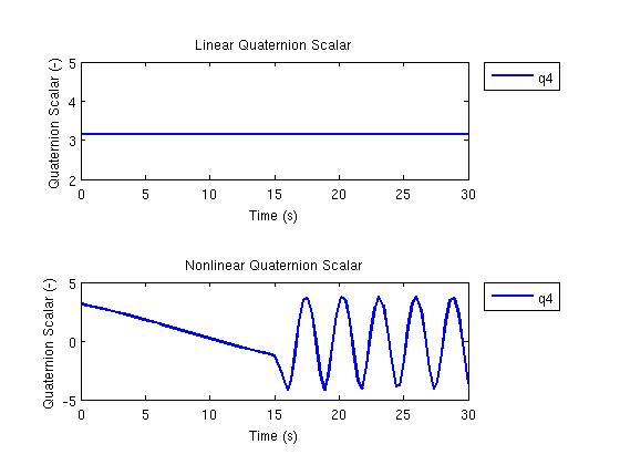
Figure 8: The linear and nonlinear responses of the quaternion scalar to the moments enacted upon the idealized rigid spacecraft model.
If you recall, the scalar quaternion component helps describe the relationship between the quaternion vector and the spacecraft's rotation about that vector (thus resulting in a final attitude for the spacecraft). Thus, it makes sense that the scalar quaternion component would mirror the vector quaternion response to some extent. The linear model of the system did not depict this relationship. However, figure 8 shows that the nonlinear model, indeed, depicts the relationship between the quaternion scalar and the quaternion vector.
Essentially, what is happening is that, as the quaternion vector moves due to the spin of the spacecraft, the final rotation about that vector which describes the spacecraft attitude changes. This relationship relates directly to the rate of spin of the spacecraft. In short, the attitude is a result of the spin of the spacecraft, which is rather intuitive. But our nonintuitive model of the system, utilizing a quaternion for a description of the attitude, has to take into account the fluctuating nature of the quaternion vector itself and, thus, the scalar quaternion fluctuates in a similar manner to the vector.
If that's confusing, don't worry too much about it. Without an actual solid model, this type of description gets to be a bit of a brain melter. But if we look at the mathematics behind the system we can relate them to the response that we are observing in a manner that makes sense. So despite the abstract description of the attitude, we can be assured that the model is performing as expected due to the underlying mathematics.
Conclusions
So what's all this mean?
Well our quest is to, eventually, develop a controller system that could damp out the potentially disastrous impact of a given moment on a spacecraft. In this model, we depicted a spacecraft's equations of motion in a very robust manner, as opposed to the sloppy approximation provided by the linearized model discussed in my first blog. Since we have a robust model that reacts in a way that makes sense, we can now begin to try to control the system.
In effect, this means that we could develop a system, like a reaction control wheel system, to damp out this kind of moment impact on a spacecraft. If we had an actual cubesat that we were planning to orbit, we could use the mass properties of that satellite to fill in this model. We could then use this model as a starting point for a control system design. The control system design process is going to be something that I expand upon in future blog posts.
However, this comparison with the linear model illustrates just how important it is to have a robust spacecraft model. The nonlinear model is significantly different from the linear model. It better reflects the physical mass properties of the system, as well as the sensitivity of the attitude to such a strong impact moment. The utilization of the quaternion to describe the attitude does, however, complicate the analysis of the system since the quaternion refers to a particular rotation about a particular vector described in the inertial frame. This is much less intuitive to deal with than something more concrete, like a series of angular rotations away from an inertial frame. However, the same mathematical nuances that make the quaternion so confusing are precisely what make it powerful. Due to the four component nature of the quaternion, the system attitude will never hit a singularity error, which is a common problem when describing the attitude via angles alone. As such, the computer on board the spacecraft can be aware of its attitude no matter what orientation it is in without throwing any, "divide by zero" faults. Thus, the quaternion is a necessary evil when dealing with spacecraft attitude dynamics.
The next step of this analysis is to start trying to control the system. We can do this by feeding the vehicle state vector back through a gain and into the input of the system. If we were actually building a spacecraft, we would essentially be coding a loop into our on board computer that forced it to calculate its total state from the previous state it was aware of. This is opposed to an open system, like that depicted here, where the computer would calculate its state entirely upon a continuous time clock without any reference to its previous state. Thus, our next blog will discuss the nature of full state feedback, and the design needed to implement such a system to control a spacecraft's attitude to keep it from spinning out of control as the one modeled here does.
Until I get that blog post up, good luck, and good hacking!
Brady C. Jackson
Comparison Script Source Code
% Uncontrolled_Linear_System.m
% Author: Brady C. Jackson
% Date: 12/05/2010
% Comments: This script will be used to initialize an Simulink model that
%           will simulate an undamped, uncontrolled linear spacecraft
%           system.

%           Prime and clear the workspace
clear;
clc;

% Build up the Linear system matrices from their components

% Make some building blocks
a = zeros(3,3);
athree = zeros(3,1);
I = eye(3,3);

% Define the initial quaternion
qfour = 1;
q = 1/2 * qfour * I;

% Define a symetric inertia matrix (can be remodeled later for realism)

J = [1.2, 0.006, 0.2 ; 0.006, 0.8, 0.005; 0.2, 0.005, 1.1];

% Define your A, B, C, and D Full-State Linear System

% Dynamics Matrix A
A = [a, a, athree; q, a, athree; athree', athree', 0];

% Inputs Matrix B
B = [inv(J); zeros(4,3)];

% Outputs vs. State Matrix C
C = [I, a, athree; a, I, athree; athree', athree', 1];

% Outputs vs. Inputs Matrix D
D = zeros(7,3);

% Check Dimensionality
Check = [A, B; C, D];
size(Check)

% Define Initial Conditions as defined by Problem 4
w = [0.1; 0.1; 0.1];
q = [0.33; 2.2; 1.768];
qfour = [3.14159];

% Define initial inputs (moment matrix) M arbitrarily
M = [5; 1.7; 2.2];

% Run Simulation Model
sim('Uncontrolled_Comparison_Sim');

% Plot Results
% Input Moments
plot(tout,u_in_lin,'Linewidth',2)
title('Input Moments')
xLim([0,30])
yLim([0,7])
xlabel('Time (s)')
ylabel('Input Moments (Nm)')
legend('X-axis Moment','Y-axis Moment','Z-axis Moment','Location','BestOutside')

% Angular Velocities
figure

subplot(2,1,1);
plot(tout,w_out_lin,'Linewidth',2)
title('Linear Angular Velocities')
xLim([0,30])
%yLim([0,7])
xlabel('Time (s)')
ylabel('Angular Velocities (rad/s)')
legend('X-axis Spin', 'Y-axis Spin', 'Z-axis Spin', 'Location', 'BestOutside')

subplot(2,1,2);
plot(tout,w_out_non,'Linewidth',2)
title('Nonlinear Angular Velocities')
xLim([0,30])
%yLim([0,7])
xlabel('Time (s)')
ylabel('Angular Velocities (rad/s)')
legend('X-axis Spin', 'Y-axis Spin', 'Z-axis Spin', 'Location', 'BestOutside')

% Quaternion Vector
figure

subplot(2,1,1);
plot(tout,q_out_lin,'Linewidth',2)
title('Linear Quaternion Vector')
xLim([0,30])
%yLim([0,7])
xlabel('Time (s)')
ylabel('Quaternion Vector Components (-)')
legend('q1', 'q2', 'q3', 'Location', 'BestOutside')

subplot(2,1,2);
plot(tout,q_out_non,'Linewidth',2)
title('Nonlinear Quaternion Vector')
xLim([0,30])
%yLim([0,7])
xlabel('Time (s)')
ylabel('Quaternion Vector Components (-)')
legend('q1', 'q2', 'q3', 'Location', 'BestOutside')

% Quaternion Scalar
figure

subplot(2,1,1);
plot(tout,q4_out_lin,'Linewidth',2)
title('Linear Quaternion Scalar')
xLim([0,30])
%yLim([0,7])
xlabel('Time (s)')
ylabel('Quaternion Scalar (-)')
legend('q4', 'Location', 'BestOutside')

subplot(2,1,2);
plot(tout,q4_out_non,'Linewidth',2)
title('Nonlinear Quaternion Scalar')
xLim([0,30])
%yLim([0,7])
xlabel('Time (s)')
ylabel('Quaternion Scalar (-)')
legend('q4', 'Location', 'BestOutside')
0 Comments
Your comment will be posted after it is approved.

 RSS Feed
