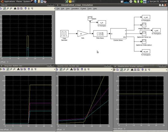
A screenshot of my workspace for modeling an uncontrolled, linearized spacecraft on orbit.
Introduction
Howdy Everyone,
This particular blog entry is going to be a throwback to some of the control systems work I did in my college days. Essentially, control systems engineering involves the design and analysis of the motion of a given system, in this case, an idealized rigid spacecraft. For any given system, or body, there is a set of equations of motion that can describe that system. Usually this involves things like translational velocity, angular velocity, translational accelerations, angular accelerations, and so on. Once the equations of motion of a body are understood, the state of the body, meaning the attitude and motion of it, can be controlled via commands to controlling devices. The process of studying these equations of motion, simulating them, and employing those simulations to develop computer code and hardware specifications is known as control systems engineering.
This particular blog entry is going to be a throwback to some of the control systems work I did in my college days. Essentially, control systems engineering involves the design and analysis of the motion of a given system, in this case, an idealized rigid spacecraft. For any given system, or body, there is a set of equations of motion that can describe that system. Usually this involves things like translational velocity, angular velocity, translational accelerations, angular accelerations, and so on. Once the equations of motion of a body are understood, the state of the body, meaning the attitude and motion of it, can be controlled via commands to controlling devices. The process of studying these equations of motion, simulating them, and employing those simulations to develop computer code and hardware specifications is known as control systems engineering.
With regards to orbital spacecraft like satellites, the development of a control subsystem for a spacecraft focuses primarily on controlling the angular rates, meaning the spin motion, and the attitude of the spacecraft. The attitude refers to the direction your spacecraft is pointing. For much of a satellite's mission, it's orbital motion is known and remains relatively steady. The only motion that needs to be actively controlled when in these states, therefore, is the pointing motion of the satellite. Orbital motion is primarily controlled when a spacecraft is transferring from one orbit to another. Thus, the first few blogs that I am going to develop regarding controls engineering are going to focus on controlling the angular motion and attitude of an ideal, rigid body satellite already on orbit.
Nomenclature
In order to define the motion of an orbiting spacecraft, as well as its attitude, I need to discuss a few terms and symbols I will be using. In order to describe the spacecraft, I will be referring to a set of body axes. These axes will represent an orthogonal Cartesian set of three axes placed somewhere on the body of our theoretical spacecraft. All of the attitudes will refer to this set of body axes. All of the angular rates of the spacecraft (spin rates, depicted as little omega or 'w') will be discussed as rates of spin about each one of these axes (x, y, and z) respectively. For a given spacecraft, the body axis can be set wherever a design engineer desires. However, it is common to place the origin of the axes as close to the spacecraft center of mass as possible, while pointing the x-axis through some primary axis. For instance, an engineer could decide to point the x-axis out of the nose of the spacecraft, in the direction that the primary communications dish is pointing.
Next, I need to introduce quaternions. A quaternion is, essentially, a mathematical construct made up of a three component vector and a scalar component. The vector portion of the quaternion describes a vector in space that can be related to the body axes of a spacecraft. The scalar portion represents the rotation about that vector that a spacecraft would need to undergo to complete a desired maneuver. Essentially, the body axes of a spacecraft can define the spacecraft attitude as a set of angles rotated through from an inertial axis set. The quaternion can represent the same rotation through a single rotation about a particular vector. Thus, the scalar and vector components of a quaternion work together to describe the attitude of a spacecraft. For the purposes of this discussion, the quaternion vector will be called 'q' while the quaternion scalar will be called 'q4.' For more information regarding quaternions you can consult Wikipedia, refer to the authoritative source on quaternions, or explore the applications quaternions have in spacecraft.
Finally, in order to describe the full state of a spacecraft, we need to refer to the mass properties of the spacecraft, meaning the moments of inertia about our chosen set of body axes. These properties can be stored in an inertia tensor which we will call 'J.' We also need to discuss whatever outside forces will be acting on our spacecraft. Thus, we will be referring to external moments enacted upon the spacecraft bus as 'M.'
Equations of Motion of a Spacecraft
Now, considering the nomenclature discussed above, we can begin to describe the state of our spacecraft with three parameters. First, we need to consider the rate of change of the angular rates of the spacecraft. This can be given as a derivative of the angular velocities, and will be referred to as w_dot. Next, we need to consider how the attitude of our spacecraft is changing. Thus, we need to consider the rates of change of our quaternion vector and quaternion scalar. These will be referred to as q_dot and q4_dot respectively. It turns out that one only needs three equations to describe the dynamics and kinematics of a rigid body in space. These are given by the three equations below.
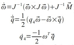
Equations 1 - 3: Equations of motion of a rigid body spacecraft given in the order of angular accelerations (w_dot), quaternion vector rates (q_dot), and the quaternion scalar rate (q4_dot).
The equations above show that our system is a nonlinear system. In other words, the rates of change of each of the state variables rely on more than just the lesser order variables themselves. So, for instance, q_dot not only relies on the lesser order q, but also q4 and w. Thus, we have a linked system where changes in one variable will induce changes in all other state variables, which will feedback around to cause changes in the first variable again. Due to the cross-linked nature of the state variables, therefore, we cannot use a simple linear model (such as an A, B, C, D state-space model) to represent the system. The coefficients in such a representation would not only contain numeric coefficients, but also, other state variables. This makes the system particularly tricky to simulate and control as a result.
Linearized Model and Equilibrium Point
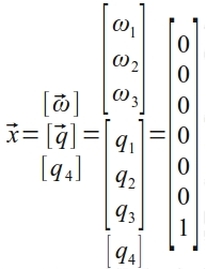
Equation 4: Equilibrium point for idealized,
rigid body spacecraft system
rigid body spacecraft system
One of the things we can do when facing a nonlinear control problem like this is simplify it where applicable. It turns out that, near an equilibrium point, nonlinear systems act like linear systems. An equilibrium point is defined as a state where a system remains stable. In other words, given no external inputs, the state variables (w, q, and q4) will hold constant. For the system described above, the state vector shown in equation 4 exists as an equilibrium point.
Knowing this to be an equilibrium point gives us the ability to, 'linearize,' the system described by the equations of motion. This requires us to take the Jacobian of the equations of motion. In other words, we need to take the derivative of each of the above equations (1 through 3) with respect to each of the state vectors (w, q, and q4). We can then plug the equilibrium point in equation 4 into the resulting equations to derive a state coefficient matrix (A) that we can employ in a linear state-space system. It is important to remember that, when utilizing this linearization method, the results will only be valid very close to the equilibrium point. The further we move from the equilibrium state, the less accurate such an approximation becomes.
Knowing this to be an equilibrium point gives us the ability to, 'linearize,' the system described by the equations of motion. This requires us to take the Jacobian of the equations of motion. In other words, we need to take the derivative of each of the above equations (1 through 3) with respect to each of the state vectors (w, q, and q4). We can then plug the equilibrium point in equation 4 into the resulting equations to derive a state coefficient matrix (A) that we can employ in a linear state-space system. It is important to remember that, when utilizing this linearization method, the results will only be valid very close to the equilibrium point. The further we move from the equilibrium state, the less accurate such an approximation becomes.
So when we take the Jacobian derivative as described above we end up with the State matrix depicted in equation 5 below.
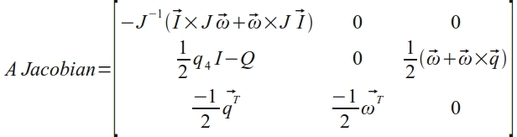
Equation 5: Jacobian derivative of the spacecraft equations of motion system.
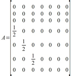
Equation 6: Linearized state matrix of an
idealized, rigid body spacecraft about
the equilibrium point depicted in equation 4.
idealized, rigid body spacecraft about
the equilibrium point depicted in equation 4.
Each of the Jacobian elements relates to each of the block derivatives of the equations of motion. So, for instance, the derivative of w_dot with respect to w yields the first element. The derivative of w_dot with respect to q yields the second element, and the derivative of q with respect to w yields the fourth element. For reference, I_vector in the equation above represents a single 3 x 1 unity vector. The I matrix (without the arrow) represents a 3 x 3 identity matrix. Q represents the cross product matrix of the q vector which has the dimensions of 3 x 3.
Once we plug the equilibrium state of the system from equation 4 we find this system simplifies to the state matrix, A, in equation 6. Notice how this linearization leaves q reliant entirely upon constant coeffecients of 1/2. This is because the zero and unity elements of the equilibrium state end up simplifying many of the equations in the Jacobian matrix. For instance, the cross products with w and q always drive to zero since the cross product of a zero vector yields a zero result. As a result, w and q4 do not respond to changes in the system itself at all. Instead, changes in these state variables will be reliant upon the input vector M, and the effects must be studied with an input matrix.
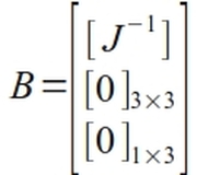
Equation 7: Input matrix for
linearized spacecraft system.
linearized spacecraft system.
Following a similar procedure to that which we used to derive A, we can take the derivative of the three equations of motion (equations 1 - 3) with respect to the input vector, or the external moments, M. This yields the B matrix of the idealized state space system depicted in equation 7. Notice that the B leaves the q and q4 rates untouched (zeros in the last 4 rows) but leaves the angular rates (w) reliant upon the mass properties matrix (top three rows). This will be important to remember later.
Finally, to round off our state-space system, we need to develop an output matrix, C, and a feedthrough matrix, D. For the purposes of our model, we are going to assume perfect observability and an output that is equal to the state vector output. Thus, the C matrix will be a 7 x 7 identity matrix. We will also be neglecting a feedthrough loop because it is unnecessary for our control system design. Thus, D will consist of a zero matrix with a 7 x 3 dimensionality. These two components are depicted in equations 8 and 9 below.
Finally, to round off our state-space system, we need to develop an output matrix, C, and a feedthrough matrix, D. For the purposes of our model, we are going to assume perfect observability and an output that is equal to the state vector output. Thus, the C matrix will be a 7 x 7 identity matrix. We will also be neglecting a feedthrough loop because it is unnecessary for our control system design. Thus, D will consist of a zero matrix with a 7 x 3 dimensionality. These two components are depicted in equations 8 and 9 below.
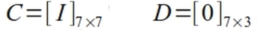
Equations 8 and 9: The Identity output matrix and the zero feedthrough matrix will suffice for our model.
So, now that we have an ideal state-space system derived to model our spacecraft near the equilibrium point, we can start to simulate the system. I employed Matlab and Simulink in order to model this system. I tried to use the open-source analysis suite of Scilab and Xcos. However, Xcos proved to be so buggy that I couldn't get the models implemented without crashing the program. Hopefully the program will mature with time. For now, however, we will be using the proprietary programs to do our analysis.
Linearized Model and Analysis
In order to model our spacecraft I utilized a script in Matlab. The script source code is posted below. Essentially, the script builds the four state space matrices that I discussed in the previous section. This is necessary because the Simulink model uses those matrices as input to simulate the system. Notice, also, that I primed a moment of inertia matrix, J. This matrix was set up as: J = [1.2, 0.006, 0.2; 0.006, 0.8, 0.005; 0.2, 0.005, 1.1] because I wanted to simulate something about the same size of a cubesat. If we define this matrix to use the units of kg * m^2 then the numerical magnitudes mostly make sense for a cubesat, which is supposed to weigh less than 1.33 kgs and only be 10 cm per edge. Thus, the largest moment arm we could have in such a system would be five times the square root of three centimeters, so the moments of inertia are about the right magnitude.
The script runs the model for 30 seconds. During this time, at about 15 seconds, a small impulse moment named 'M' in the script is input to the model using a pulse generator. The input moment is applied to the model for 1 second at 15 seconds into the simulation. This is meant to simulate an off axis micro meteor impact, or, perhaps, it could simulate a small, temporary leak in a fuel line. Either way, I applied a moment input vector of [5.0; 1.7; 2.2] Nm about my body axes. This gave me the opportunity to study the response of a linearized system given some sort of unexpected external event. The Simulink model I used to simulate this response is depicted in Figure 1.
The script runs the model for 30 seconds. During this time, at about 15 seconds, a small impulse moment named 'M' in the script is input to the model using a pulse generator. The input moment is applied to the model for 1 second at 15 seconds into the simulation. This is meant to simulate an off axis micro meteor impact, or, perhaps, it could simulate a small, temporary leak in a fuel line. Either way, I applied a moment input vector of [5.0; 1.7; 2.2] Nm about my body axes. This gave me the opportunity to study the response of a linearized system given some sort of unexpected external event. The Simulink model I used to simulate this response is depicted in Figure 1.
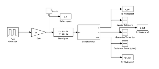
Figure 1: Model of an ideal, rigid body, linearized spacecraft undergoing a small moment impulse at t = 15 seconds.
You may notice that I branch off all of my outputs to two different sinks. First, I piped all of my state outputs (w, q, and q4) into scopes to help me monitor the model real-time and debug the model. Second, I piped the same outputs back to my workspace so that they could be plotted up as figures. This is reflected in the latter part of my run script.
Finally, I also plotted and monitored the input moments to the linear plant (State-Space block). These input moments are reflected in figure 2.
Finally, I also plotted and monitored the input moments to the linear plant (State-Space block). These input moments are reflected in figure 2.
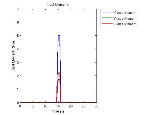
Figure 2: Moments input into the system at t = 15 seconds. M = [5.0; 1.7; 2.2] Nm.
As you can see, the three separate moments (one about each axis) occur as I planned at 15 seconds. So now let's study the response of the system to this impulse. First, we'll check out the change in the angular velocities about each of the three axes. See figure 3.
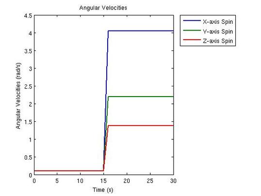
Figure 3: Angular velocity response to input moment on linearized spacecraft system.
Studying figure 3 we start to see some interesting patterns. First, the angular velocities don't start out at zero. This is because I defined an initial angular velocity vector of 0.1 rad/s around each axis. This is meant to simulate a slow spin of our cubesat, maybe for thermal control purposes or something. Next, we study the jump in rates at 15 seconds. Notice how the three spin rates leap proportionally to the moments input on each axis. Studying our state-space matrices from above reveals the reason for this. Essentially, the w vector is reliant entirely upon the mass properties matrix and the input moments. Since the first three rows of our A matrix are zeroed out for our linear approximation, there is no response in w with respect to changes in the rest of the state variables. It makes sense, therefore, that the spin rates would jump due only to the input moments.
This also starts to depict why this sort of analysis is known as a linearization technique. The response to the inputs is rather 1 dimensional. As the moment input to the system increases, the angular rates increase proportionally. That's pretty much the definition of a linear response. So let's see if that trend holds true for the quaternion vector. See figure 4..
This also starts to depict why this sort of analysis is known as a linearization technique. The response to the inputs is rather 1 dimensional. As the moment input to the system increases, the angular rates increase proportionally. That's pretty much the definition of a linear response. So let's see if that trend holds true for the quaternion vector. See figure 4..
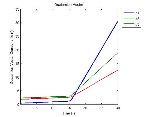
Figure 4: Quaternion response to input moment on linearized spacecraft system.
Notice how the quaternion vector is slightly changing right form the start. This is due to the initial spin implemented on the spacecraft discussed in the previous section. As the spacecraft spins, the attitude of the spacecraft changes. That makes sense. But what happens when the moment impulse occurs? Well, we see the quaternion vector components erupt in magnitude as they increase into oblivion. What causes this?
If we observe the A matrix of our system, we note that the q vector response is coupled, entirely, to the spin rates (w vector) of our spacecraft. Now, there is a 1/2 coefficient to lessen the drama of the response, but, we still see that as the spin rates increase due to the moment input, the quaternion responds in kind by spinning all to hell. In the end, the induced moment causes our spacecraft to spin out of control in such a manner that it becomes useless. If our spacecraft is spinning uncontrollably, then we can't do much useful science with it can we? So this model starts to show us how disastrous something like a micro meteorite impact on a cubesat could be.
But let's move on and see how the quaternion scalar is impacted by such a moment on the spacecraft. see figure 5.
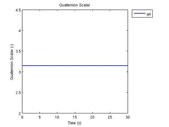
Figure 5: Quaternion scalar response to input moment on linearized spacecraft.
Well that's a pretty uneventful response isn't it? If we revisit out state space system we will notice that the q4 response row gets zeroed our in both the A and the B matrices (row 7). As a result, no matter what we do to the system, we cannot solicit a response in the q4 response. And, thus, we see the limitations of linearized approximation models. Really, in order to understand the behavior of a spacecraft due to an imparted momentum like the one we simulated, we need to fully model the nonlinear body of equations depicted in equations 1 through 3.
Once we properly simulate the system, then we can begin trying to control the system via feedback loops and various controller methods. Luckily for you, I am going to be furthering this analysis in exactly this manner over the next few weeks. First, I will model the nonlinear spacecraft equations and compare them to this model for reference. Next, I am going to show how you can utilize a feedback loop with a simple gain imparted on your state signal (via something like an op amp) to damp out and control your response to a moment like the one we simulated here.
Until then, however, I hope you enjoyed this brief introduction to spacecraft control systems. One interesting thing to note is that this type of analysis can be carried into any system, including things like robotic joints and rover motions, or, hell, even cybernetic enhancements to the human body. In other words, as long as the equations of motion of a system can be determined, the analysis and control methods I am discussing will be applicable to those systems. So you can see how exciting this field of engineering and analysis can be. As I progress through the means of controlling a system via simulation, hopefully I will start to apply some of the same control techniques to actual hardware, like my Ardie platform. This type of project is a ways off in the future, but I look forward to bridging that gap between theory and reality.
So, until next time, good luck and good hacking!
Brady C. Jackson
Matlab Primer Script Source Code
 % Uncontrolled_Linear_System.m
 % Author: Brady C. Jackson
 % Date: 12/05/2010
 % Comments: This script will be used to initialize a Simulink model that
 %           will simulate an undamped, uncontrolled linear spacecraft
 %           system.

 %           Prime and clear the workspace

 clear;
 clc;

 % Build up the Linear system matrices from their components
 % Make some building blocks
 a = zeros(3,3);
 athree = zeros(3,1);
 I = eye(3,3);

 % Define the initial quaternion
 qfour = 1;
 q = 1/2 * qfour * I;

 % Define a symetric inertia matrix (can be remodeled later for realism)
 J = [1.2, 0.006, 0.2 ; 0.006, 0.8, 0.005; 0.2, 0.005, 1.1];

 % Define your A, B, C, and D Full-State Linear System
 % Dynamics Matrix A
 A = [a, a, athree; q, a, athree; athree', athree', 0];

 % Inputs Matrix B
 B = [inv(J); zeros(4,3)];

 % Outputs vs. State Matrix C
 C = [I, a, athree; a, I, athree; athree', athree', 1];

 % Outputs vs. Inputs Matrix D
 D = zeros(7,3);

 % Check Dimensionality
 Check = [A, B; C, D];
 size(Check)

 % Define Initial Conditions as defined by Problem 4
 w = [0.1; 0.1; 0.1];
 q = [0.33; 2.2; 1.768];
 qfour = [3.14159];

 % Define initial inputs (moment matrix) M arbitrarily
 M = [5; 1.7; 2.2];

 % Run Simulation Model
 sim('Uncontrolled_Linear_Simulation');

 % Plot Results
 % Input Moments
 plot(tout,u_in,'Linewidth',2)
 title('Input Moments')
 xLim([0,30])
 yLim([0,7])
 xlabel('Time (s)')
 ylabel('Input Moments (Nm)')
 legend('X-axis Moment','Y-axis Moment','Z-axis Moment','Location','BestOutside')

 % Angular Velocities
 figure

 plot(tout,w_out,'Linewidth',2)
 title('Angular Velocities')
 xLim([0,30])
 %yLim([0,7])
 xlabel('Time (s)')
 ylabel('Angular Velocities (rad/s)')
 legend('X-axis Spin', 'Y-axis Spin', 'Z-axis Spin', 'Location', 'BestOutside')

 % Quaternion Vector
 figure

 plot(tout,q_out,'Linewidth',2)
 title('Quaternion Vector')
 xLim([0,30])
 %yLim([0,7])
 xlabel('Time (s)')
 ylabel('Quaternion Vector Components (-)')
 legend('q1', 'q2', 'q3', 'Location', 'BestOutside')

 % Quaternion Scalar
 figure

 plot(tout,q4_out,'Linewidth',2)
 title('Quaternion Scalar')
 xLim([0,30])
 %yLim([0,7])
 xlabel('Time (s)')
 ylabel('Quaternion Scalar (-)')
 legend('q4', 'Location', 'BestOutside')

 RSS Feed
